Lower Bound Theory Concept is based upon the calculation of minimum time that is required to execute an algorithm is known as a lower bound theory or Base Bound Theory.

Lower Bound Theory uses a number of methods/techniques to find out the lower bound.

Concept/Aim: The main aim is to calculate a minimum number of comparisons required to execute an algorithm.

Techniques:

The techniques which are used by lower Bound Theory are:

1. Comparisons Trees.
2. Oracle and adversary argument
3. State Space Method

1. Comparison trees:

In a comparison sort, we use only comparisons between elements to gain order information about an input sequence (a1; a2......an).

Given a_i,a_j from (a₁, a₂.....a_n)We Perform One of the Comparisons

• a_i < a_j    less than
• a_i ≤ a_j    less than or equal to
• a_i > a_j    greater than
• a_i ≥ a_j    greater than or equal to
• a_i = a_j    equal to

To determine their relative order, if we assume all elements are distinct, then we just need to consider a_i ≤ a_j '=' is excluded &, ≥,≤,>,< are equivalent.

Consider sorting three numbers a1, a2, and a3. There are 3! = 6 possible combinations:

1. (a1, a2, a3), (a1, a3, a2),  
2. (a2, a1, a3), (a2, a3, a1)  
3. (a3, a1, a2), (a3, a2, a1)  

The Comparison based algorithm defines a decision tree.

Decision Tree: A decision tree is a full binary tree that shows the comparisons between elements that are executed by an appropriate sorting algorithm operating on an input of a given size. Control, data movement, and all other conditions of the algorithm are ignored.

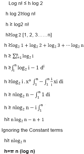
In a decision tree, there will be an array of length n.

So, total leaves will be n! (I.e. total number of comparisons)

If tree height is h, then surely

    n! ≤2n (tree will be binary)

Taking an Example of comparing a1, a2, and a3.

Left subtree will be true condition i.e. a_i ≤ a_j

Right subtree will be false condition i.e. a_i >a_j

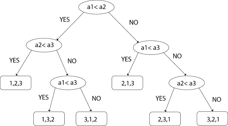Fig: Decision Tree

So from above, we got

N! ≤2n   

Taking Log both sides

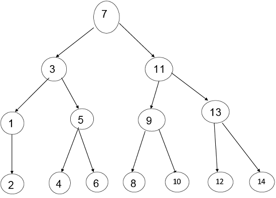
Comparison tree for Binary Search:

Example: Suppose we have a list of items according to the following Position:

1. 1,2,3,4,5,6,7,8,9,10,11,12,13,14  

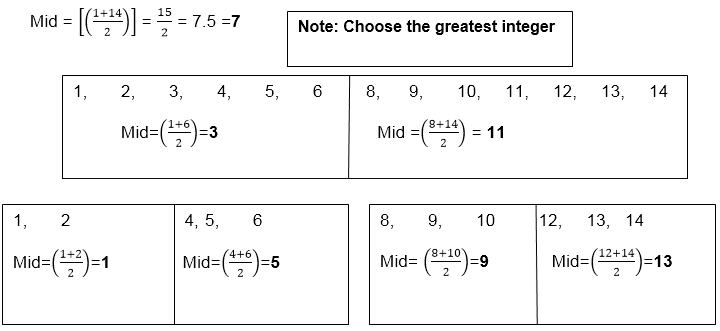And the last midpoint is:

1. 2,  4,  6,  8,  10, 12, 14  

Thus, we will consider all the midpoints and we will make a tree of it by having stepwise midpoints.

The Bold letters are Mid-Points Here

According to Mid-Point, the tree will be:

Step1: Maximum number of nodes up to k level of the internal node is 2^k-1

For Example

 2k-1
 23-1= 8-1=7
Where k = level=3

Step2: Maximum number of internal nodes in the comparisons tree is n!

Note: Here Internal Nodes are Leaves.

Step3: From Condition1 & Condition 2 we get

N! ≤ 2k-1
 14 < 15
 Where N = Nodes

Step4: Now, n+1 ≤ 2^k

Here, Internal Nodes will always be less than 2^k in the Binary Search.

Step5:

n+1<= 2k
   Log (n+1) = k log 2
 k >= 

k >=log

2(n+1)

Step6:

1. T (n) = k  

Step7:

T (n) >=log2(n+1)

Here, the minimum number of Comparisons to perform a task of the search of n terms using Binary Search

2. Oracle and adversary argument:

Another technique for obtaining lower bounds consists of making use of an "oracle."

Given some model of estimation such as comparison trees, the oracle tells us the outcome of each comparison.

In order to derive a good lower bound, the oracle efforts it's finest to cause the algorithm to work as hard as it might.

It does this by deciding as the outcome of the next analysis, the result which matters the most work to be needed to determine the final answer.

And by keeping step of the work that is finished, a worst-case lower bound for the problem can be derived.

Example: (Merging Problem) given the sets A (1: m) and B (1: n), where the information in A and in B are sorted. Consider lower bounds for algorithms combining these two sets to give an individual sorted set.

Consider that all of the m+n elements are specific and A (1) < A (2) < ....< A (m) and B (1) < B (2) < ....< B (n).

Elementary combinatory tells us that there are C ((m+n), n)) ways that the A's and B's may merge together while still preserving the ordering within A and B.

Thus, if we need comparison trees as our model for combining algorithms, then there will be C ((m+n), n)) external nodes and therefore at least log C ((m+n), m) comparisons are needed by any comparison-based merging algorithm.

If we let MERGE (m, n) be the minimum number of comparisons used to merge m items with n items then we have the inequality

1. Log C ((m+n), m) MERGE (m, n) m+n-1.   

The upper bound and lower bound can get promptly far apart as m gets much smaller than n.

3. State Space Method:

1. State Space Method is a set of rules that show the possible states (n-tuples) that an algorithm can assume from a given state of a single comparison.

2. Once the state transitions are given, it is possible to derive lower bounds by arguing that the finished state cannot be reached using any fewer transitions.

3. Given n distinct items, find winner and loser.

4. Aim: When state changed count it that is the aim of State Space Method.

5. In this approach, we will count the number of comparison by counting the number of changes in state.

6. Analysis of the problem to find out the smallest and biggest items by using the state space method.

7. State: It is a collection of attributes.

8. Through this we sort out two types of Problems:

1. Find the largest & smallest element from an array of elements.
2. To find out largest & second largest elements from an array of an element.

9. For the largest item, we need 7 comparisons and what will be the second largest item?

Now we count those teams who lose the match with team A 
    Teams are: B, D, and E
So the total no of comparisons are: 7
Let n is the total number of items, then
    Comparisons = n-1 (to find the biggest item) 
No of Comparisons to find out the 2nd biggest item = log2n-1

10. In this no of comparisons are equal to the number of changes of states during the execution of the algorithm.

Example: State (A, B, C, D)

1. No of items that can never be compared.
2. No of items that win but never lost (ultimate winner).
3. No of items that lost but never win (ultimate loser)
4. No of items who sometimes lost & sometimes win.

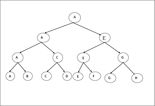Firstly, A, B compare out or match between them. A wins and in C, D.C wins and so on. We can assume that B wins and so on. We can assume that B wins in place of A it can be anything depending on our self.

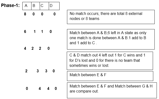In Phase-1 there are 4 states

If the team is 8 then 4 states

As if n team the n/2 states.

4 is Constant in C-State as B, D, F, H are lost teams that never win.

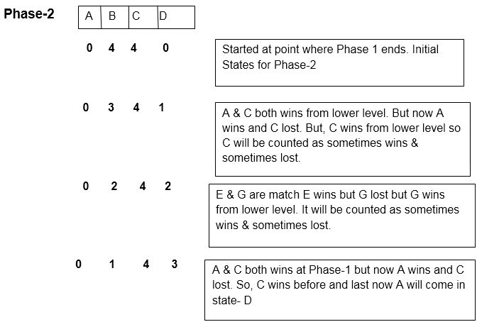
Thus there are 3 states in Phase-2,

If n is 8 then states are 3

If n teams that are states.

Phase-3: This is a Phase in which teams which come under C-State are considered and there will be matches between them to find out the team which is never winning at all.

In this Structure, we are going to move upward for denoting who is not winning after the match.

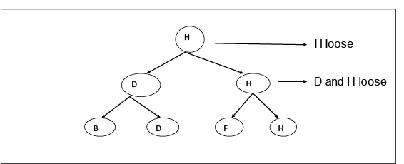Here H is the team which is never winning at all. By this, we fulfill our second aim to.

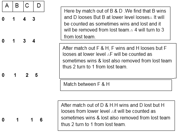Thus there are 3 states in Phase -3

If n teams that are  states

Note: the total of all states value is always equal to 'n'.

Thus, by adding all phase's states we will get:-

Phase1 + Phase 2 + Phase 3

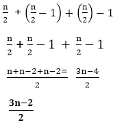Suppose we have 8 teams then 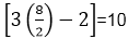states are there (as minimum) to find out which one is never wins team.

Thus, Equation is:

Lower bound (L (n)) is a property of the particular issue i.e. the sorting problem, matrix multiplication not of any particular algorithm solving that problem.

Lower bound theory says that no calculation can carry out the activity in less than that of (L (n)) times the units for arbitrary inputs i.e. that for every comparison based sorting algorithm must take at least L (n) time in the worst case.

L (n) is the base overall conceivable calculation which is greatest finished.

Trivial lower bounds are utilized to yield the bound best alternative is to count the number of elements in the problems input that must be prepared and the number of output items that need to be produced.

The lower bound theory is the method that has been utilized to establish the given algorithm in the most efficient way which is possible. This is done by discovering a function g (n) that is a lower bound on the time that any algorithm must take to solve the given problem. Now if we have an algorithm whose computing time is the same order as g (n) , then we know that asymptotically we cannot do better.

If f (n) is the time for some algorithm, then we write f (n) = Ω (g (n)) to mean that g (n) is the lower bound of f (n) . This equation can be formally written, if there exists positive constants c and n0 such that |f (n)| >= c|g (n)| for all n > n0. In addition for developing lower bounds within the constant factor, we are more conscious of the fact to determine more exact bounds whenever this is possible.

Deriving good lower bounds is more challenging than arrange efficient algorithms. This happens because a lower bound states a fact about all possible algorithms for solving a problem. Generally, we cannot enumerate and analyze all these algorithms, so lower bound proofs are often hard to obtain.